LAB 06 · 颜色干预:视图、投影与读出
主线阅读与优先实验
真实RGB对比训练、唯一指定增强变化、h/z形状与颜色读出
对应课堂(3 页)
可先阅读已有结果,再决定是否运行。重算时请核对各节记录的数据、参数、环境与日期。
学习路径: 视图、投影头与历史字典
希望模型忽略颜色,会怎样改变它对形状与颜色的判断?
先看同一源图的保色/换色视图,写下对两项任务的预测;再看真实训练的h/z读出表。颜色增强改善了本次形状读出,同时削弱颜色读出;h并不是保证保留信息的保险箱。
本册的重点代码是views、info_nce和冻结评价;开头二维向量只是可行构造。模型、数据和完整训练均保留,运行从新内核顺序开始。表格与图标明已有本地结果,后文另列旧云端复核,不合并成同一次测量。
产出一张两行对照:预测的变化、观察到的变化,以及你认为可继续检验的解释。P13和对应证据段落与本册同题。只有想检查候选从哪里来,再接LAB 07的历史字典。
热身:一种可行构造,尚未学习
四个向量表示两种颜色和两种亮度。令 z 等于两个通道之和,那么红与蓝可以得到相同 z。这个例子只证明“投影可以丢颜色”,没有证明训练必然如此,更没有证明 h 永远保留颜色。
展开完整实现代码
import os, tempfile
LAB_WORKDIR = tempfile.mkdtemp(prefix='lecture03-')
os.chdir(LAB_WORKDIR)
print('Ephemeral experiment workspace ready')
import numpy as np
h=np.array([[1.,0.],[.7,0.],[0.,1.],[0.,.7]])
y=np.array([0,0,1,1]);z=h.sum(1,keepdims=True)
print('h shape',h.shape,'z shape',z.shape)
print('h color readout',np.argmax(h,1).tolist(),'z',z.ravel().tolist())
print('This is a hand-constructed projection, not learned features.')运行准备与结果身份
本册包含全部生成数据、模型、损失、优化与评价代码。按顺序在新内核运行;不读另一册的变量,不需要下载图像或预训练权重。依赖 Python 3.12、NumPy、matplotlib、scikit-learn 和 CPU PyTorch。本次实际版本见输出 JSON;若环境缺少 PyTorch,先运行 python -m pip install torch==2.14.0 --index-url https://download.pytorch.org/whl/cpu,再启动内核。NumPy、matplotlib、scikit-learn 可用 python -m pip install numpy matplotlib scikit-learn 安装。
下方表格和静态图来自 2026-09-22 本地 CPU 完整训练;它们不是原来的数值热身输出,也不代表 Deepnote 云端已重跑。运行本册会另建 lab06-notebook-output,保存 inputs.npz、config.json、权重、图与 results.json。CPU 时间受机器负载影响;本次每册约 10–25 秒,不能当作跨设备速度基准。单种子、小任务的结果用来检验路径和对照,不作方法排名。
展开完整实现代码
"""CPU image contrastive experiment. No class/color label enters pretraining."""
from pathlib import Path
import copy, hashlib, json, os, platform, time
import numpy as np
import torch
from torch import nn
from torch.nn import functional as F
from sklearn.neighbors import KNeighborsClassifier
from sklearn.linear_model import LogisticRegression
from sklearn.pipeline import make_pipeline
from sklearn.preprocessing import StandardScaler
import matplotlib
matplotlib.use('Agg')
import matplotlib.pyplot as plt

torch.set_num_threads(2)
SEED=20260922

SOURCE_SHA256='09bbb32bb5502db3535d89efec2045ffcd85c249b49f622390f12875060845d4'
print("source",SOURCE_SHA256,"torch",torch.__version__)从一张图到两个视图
生成 840 张 16×16 RGB 图,600 张训练、240 张保留,每个“形状×颜色”组合各 100/40 张。位置、尺度、强度和背景噪声独立变化,源图 ID 在两侧不重叠;先分源图,再在线产生增强,不能把同一源图的两个增强分到训练和评价。
两个条件共用数据、初始化、批顺序、优化器和随机数流。共同增强是每图平移 ±1 像素、亮度乘以 0.8–1.2、添加标准差 0.025 的噪声。swap-hue 额外以 50% 概率独立交换每个视图的 R/B 通道;keep-hue 不交换。相同随机数仍被消耗,所以不是意外改变了其他增强。
生成器知道标签,以便定义任务和分层采样;预训练函数只接收图像和训练 ID,没有读取形状或颜色标签。
展开完整实现代码
def make_data(seed=SEED):
    rng=np.random.default_rng(seed)
    yy,xx=np.mgrid[:16,:16]
    images=[]; shape=[]; color=[]; split=[]
    # Stratified before view construction. One independently generated source per ID.
    for s in range(3):
        for c in range(2):
            for i in range(140):
                cx,cy=rng.uniform(6,10,2); r=rng.uniform(3.0,4.7)
                dx,dy=xx-cx,yy-cy
                if s==0: mask=dx*dx+dy*dy<=r*r
                elif s==1: mask=np.maximum(abs(dx),abs(dy))<=r
                else: mask=abs(dx)+abs(dy)<=r*1.35
                # Red and blue have equal channel sums: grayscale erases hue by design.
                rgb=np.array([.9,.15,.15] if c==0 else [.15,.15,.9])
                bg=rng.uniform(.015,.075,(16,16,1))
                im=np.where(mask[...,None],rgb*rng.uniform(.8,1),bg)
                im+=rng.normal(0,.012,im.shape)
                images.append(np.clip(im,0,1).transpose(2,0,1))
                shape.append(s); color.append(c); split.append(0 if i<100 else 1)
    x=np.asarray(images,dtype='float32'); split=np.asarray(split)
    ids=np.arange(len(x)); train=ids[split==0]; test=ids[split==1]
    assert set(train).isdisjoint(test)
    assert len({hashlib.sha256(v.tobytes()).hexdigest() for v in x})==len(x)
    return torch.from_numpy(x),np.asarray(shape),np.asarray(color),train,test

def views(x, destroy_color=False):
    # Independent transforms of each source; no labels/scene attributes are read.
    a=x.clone(); n=len(a)
    shifts=torch.randint(-1,2,(n,2))
    for i,(dy,dx) in enumerate(shifts.tolist()):
        a[i]=torch.roll(a[i],(dy,dx),(-2,-1))
    a=a*torch.empty(n,1,1,1).uniform_(.8,1.2)
    a=a+torch.randn_like(a)*.025
    # The ablation changes only the hue swap. Every run consumes this RNG draw.
    swap=torch.rand(n)<.5
    if destroy_color: a[swap]=a[swap][:,[2,1,0]]
    return a.clamp(0,1)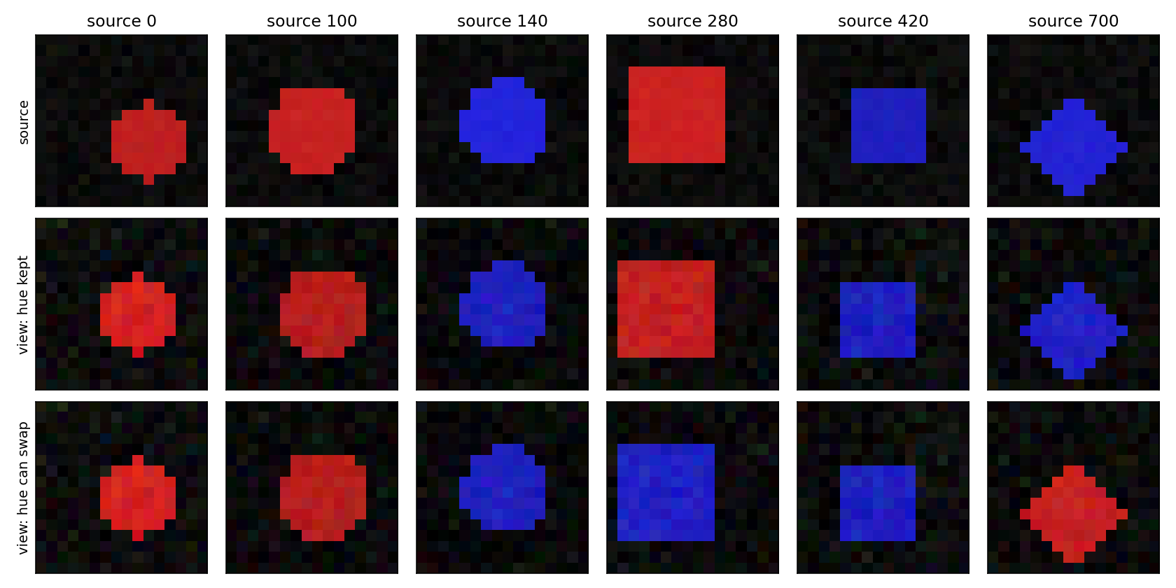
图中每列来自同一源图;最下行可以改变红蓝,但形状轮廓不变。正式训练每张源图产生两个独立视图。图是已运行基准的样例,不是为了展示目标效果而绘制的模型输出。
h 与 z:目标作用在哪一层?
编码器 f 的三层卷积将 B×3×16×16 变成 B×24×4×4,再线性读出 h∈R⁴⁸。投影头 g 是 48→48→24 的两层 MLP,中间有 ReLU。损失作用于归一化的 z=g(h),冻结评价分别读取 h 和 z。
每批 N=60 个源图产生 2N 个向量。对第 i 个视图,另一个同源视图 j 是唯一正例:
分母去掉自己,包含正例和其他源图的两视图;对 120 个锚点平均。其他源图可能恰好也是红圆,仍被当作负例:这是按源图身份定义的实例目标,未必完全符合形状类别。梯度从 z 经过投影头返回卷积编码器,所以投影头不构成阻止 h 丢信息的隔离墙。
展开完整实现代码
class ImageEncoder(nn.Module):
    def __init__(self):
        super().__init__()
        self.conv=nn.Sequential(nn.Conv2d(3,12,3,padding=1),nn.ReLU(),
          nn.Conv2d(12,24,3,stride=2,padding=1),nn.ReLU(),
          nn.Conv2d(24,24,3,stride=2,padding=1),nn.ReLU())
        self.readout=nn.Linear(24*4*4,48)
    def forward(self,x): return self.readout(self.conv(x).flatten(1))

class ContrastiveModel(nn.Module):
    def __init__(self):
        super().__init__(); self.encoder=ImageEncoder()
        self.projector=nn.Sequential(nn.Linear(48,48),nn.ReLU(),nn.Linear(48,24))
    def forward(self,x):
        h=self.encoder(x); z=self.projector(h)
        return h,z

def info_nce(z1,z2,tau=.2):
    z=F.normalize(torch.cat([z1,z2]),dim=1); n=len(z1)
    logits=z@z.T/tau
    logits=logits.masked_fill(torch.eye(2*n,dtype=torch.bool),-1e9)
    positive=(torch.arange(2*n)+n)%(2*n)
    return F.cross_entropy(logits,positive)

def train_simclr(initial,x,train,destroy_color,epochs=40):
    # Equal initialization, minibatch ordering, optimizer, steps, and RNG streams.
    torch.manual_seed(SEED+1)
    model=copy.deepcopy(initial); opt=torch.optim.Adam(model.parameters(),lr=.002)
    history=[]; before=next(model.encoder.parameters()).detach().clone()
    for epoch in range(epochs):
        model.train(); losses=[]
        for ids in torch.as_tensor(train)[torch.randperm(len(train))].split(60):
            batch=x[ids]; a,b=views(batch,destroy_color),views(batch,destroy_color)
            loss=info_nce(model(a)[1],model(b)[1])
            opt.zero_grad(); loss.backward(); opt.step(); losses.append(float(loss.detach()))
        history.append(float(np.mean(losses)))
    delta=float((next(model.encoder.parameters()).detach()-before).norm())
    assert delta>0
return model,history,delta冻结评价回答另一个问题
训练完成后对未增强的图像提取特征,编码器不再更新。h、z 先各自 L2 归一化;余弦 5-NN 只把 600 张训练图及其标签作为参考库,在 240 张保留图上预测。另做线性读出:标准化参数和 LogisticRegression 都只拟合训练特征,C=1 固定;没有用保留集选 epoch、k 或正则化。
随机基线是训练前完全相同的网络权重。随机卷积也会保留像素、边缘和颜色信息,因此机会水平不是唯一合理基线。固定输入只交换 R/B 后的余弦相似度是另一项干预;较高相似度本身不能证明颜色不可读,必须和读出共同看。
展开完整实现代码
def evaluate(model,x,ys,yc,train,test):
    model.eval()
    with torch.no_grad(): h,z=model(x)
    scores={}
    for space,features in [('h',h),('z',z)]:
        a=F.normalize(features,dim=1).numpy()
        for target,y in [('shape',ys),('color',yc)]:
            knn=KNeighborsClassifier(n_neighbors=5,metric='cosine')
            knn.fit(a[train],y[train])
            # Standardization and classifier fit use TRAIN only; test used once for reporting.
            linear=make_pipeline(StandardScaler(),LogisticRegression(C=1,max_iter=1000))
            linear.fit(a[train],y[train])
            scores[f'{space}_{target}_knn']=float(knn.score(a[test],y[test]))
            scores[f'{space}_{target}_linear']=float(linear.score(a[test],y[test]))
    with torch.no_grad():
        # Counterfactual hue swap only: same geometry and pixels, channels exchanged.
        ah,az=model(x[test][:,[2,1,0]])
        for space,original,other in [('h',h[test],ah),('z',z[test],az)]:
            scores[f'{space}_hue_swap_cosine']=float(F.cosine_similarity(original,other).mean())
    return scores

def moco_warmup():
    q=np.array([1.,0.]); keys=np.array([[.8,.2],[0.,1.],[-1.,0.]])
    keys/=np.linalg.norm(keys,axis=1,keepdims=True)
    probs={}
    for T in [.1,.5]:
        s=keys@q/T; p=np.exp(s-s.max());p/=p.sum();probs[str(T)]=p.tolist()
    queue=['a','b','c','d']; queue=(queue+['e','f'])[-4:]
    ema=.9*np.array([0.,2.])+.1*np.array([2.,4.])
    assert queue==['c','d','e','f']; assert np.allclose(ema,[.2,2.2])
    return {'temperature_probabilities':probs,'FIFO':queue,'EMA':ema.tolist()}

def train_moco(initial,x,train,epochs=15):
    # Small genuine image implementation: query grads, detached EMA keys, FIFO negatives.
    torch.manual_seed(SEED+2)
    query=copy.deepcopy(initial); key=copy.deepcopy(initial)
    for p in key.parameters(): p.requires_grad=False
    opt=torch.optim.Adam(query.parameters(),lr=.002)
    queue=torch.empty((0,24)); queue_ids=torch.empty(0,dtype=torch.long)
    history=[]; trace=[]; m=.95; capacity=240
    before=next(query.encoder.parameters()).detach().clone()
    for epoch in range(epochs):
        losses=[]
        for ids in torch.as_tensor(train)[torch.randperm(len(train))].split(60):
            a,b=views(x[ids]),views(x[ids])
            q=F.normalize(query(a)[1],dim=1)
            with torch.no_grad():
                for pk,pq in zip(key.parameters(),query.parameters()):pk.mul_(m).add_(pq,alpha=1-m)
                k=F.normalize(key(b)[1],dim=1)
            # Warmup uses detached current keys. Later batches use a real FIFO dictionary.
            if not len(queue):
                logits=q@k.T/.2; labels=torch.arange(len(ids))
                loss=F.cross_entropy(logits,labels)
            else:
                positive=(q*k).sum(1,keepdim=True)
                negative=q@queue.T
                # A source already in queue is NOT treated as its own negative.
                negative=negative.masked_fill(ids[:,None]==queue_ids[None,:],-1e9)
                logits=torch.cat([positive,negative],dim=1)/.2
                loss=F.cross_entropy(logits,torch.zeros(len(ids),dtype=torch.long))
            opt.zero_grad();loss.backward();opt.step()
            with torch.no_grad():
                queue=torch.cat([queue,k])[-capacity:];queue_ids=torch.cat([queue_ids,ids])[-capacity:]
            losses.append(float(loss.detach()))
            if len(trace)<5:trace.append({'step':len(trace),'queue_size':len(queue),'first_source_id':int(queue_ids[0]),'last_source_id':int(queue_ids[-1])})
        history.append(float(np.mean(losses)))
    assert all(p.grad is None for p in key.parameters())
    return query,key,queue,queue_ids,history,trace,float((next(query.encoder.parameters()).detach()-before).norm())

def plot_results(out,x,initial,models,results,histories):
    fig,ax=plt.subplots(3,6,figsize=(12,6))
    ids=[0,100,140,280,420,700]
    torch.manual_seed(SEED+6)
    for j,i in enumerate(ids):
        ax[0,j].imshow(x[i].permute(1,2,0));ax[0,j].set_title(f'source {i}')
        paired_state=torch.get_rng_state()
        for row,erase in [(1,False),(2,True)]:
            torch.set_rng_state(paired_state)
            ax[row,j].imshow(views(x[i:i+1],erase)[0].permute(1,2,0))
    for row,label in enumerate(['source','view: hue kept','view: hue can swap']):ax[row,0].set_ylabel(label)
    for a in ax.flat:a.set_xticks([]);a.set_yticks([])
    fig.tight_layout();fig.savefig(out/'views.png',dpi=140);plt.close(fig)
    fig,axes=plt.subplots(1,3,figsize=(14,4))
    for name,hist in histories.items():axes[0].plot(np.arange(1,len(hist)+1),hist,label=name)
    axes[0].set(xlabel='epoch',ylabel='InfoNCE (batch mean)',title='Training objective');axes[0].legend(fontsize=8)
    names=list(results)
    for ax,task in zip(axes[1:],['shape','color']):
        pos=np.arange(len(names)); width=.34
        for off,space in [(-width/2,'h'),(width/2,'z')]:
            ax.bar(pos+off,[results[n][f'{space}_{task}_knn'] for n in names],width,label=space)
        ax.set_xticks(pos,names,rotation=20);ax.set_ylim(0,1.05);ax.set_title(f'Frozen cosine 5-NN: {task}')
        ax.set_ylabel('held-out accuracy');ax.legend()
    fig.tight_layout();fig.savefig(out/'training-and-probes.png',dpi=140);plt.close(fig)

def run_contrastive(out_dir='lab06-output',mode='color'):
    started=time.time();out=Path(out_dir);out.mkdir(parents=True,exist_ok=True)
    torch.manual_seed(SEED)
    x,ys,yc,train,test=make_data()
    np.savez_compressed(out/'inputs.npz',images=x.numpy(),shape=ys,color=yc,train_ids=train,test_ids=test)
    initial=ContrastiveModel(); torch.save(initial.state_dict(),out/'random-init.pt')
    results={'random':evaluate(initial,x,ys,yc,train,test)};histories={};models={};deltas={}
    if mode=='color':
        for name,erase in [('keep-hue',False),('swap-hue',True)]:
            model,hist,delta=train_simclr(initial,x,train,erase)
            results[name]=evaluate(model,x,ys,yc,train,test);histories[name]=hist;models[name]=model;deltas[name]=delta
            torch.save(model.state_dict(),out/f'{name}.pt')
    else:
        model,hist,delta=train_simclr(initial,x,train,False)
        results['simclr']=evaluate(model,x,ys,yc,train,test);histories['simclr']=hist;models['simclr']=model;deltas['simclr']=delta
        torch.save(model.state_dict(),out/'simclr.pt')
        query,key,queue,queue_ids,hist,trace,delta=train_moco(initial,x,train)
        results['moco-toy']=evaluate(query,x,ys,yc,train,test);histories['moco-toy']=hist;models['moco-toy']=query;deltas['moco-toy']=delta
        torch.save({'query':query.state_dict(),'key':key.state_dict(),'queue':queue,'queue_ids':queue_ids},out/'moco-toy.pt')
        (out/'queue-trace.json').write_text(json.dumps(trace,indent=2))
    config={'seed':SEED,'mode':mode,'image_shape':[3,16,16],'train_n':len(train),'test_n':len(test),'batch_size':60,'epochs_simclr':40,'epochs_moco':15,'tau':.2,'adam_lr':.002,'h_dim':48,'z_dim':24,'labels_used_only_for_probes':True,'knn':{'k':5,'metric':'cosine'},'linear_probe':{'regularization_C':1,'standardizer_fit':'train-only'},'test_tuning':'none; fixed protocol before first run'}
    (out/'config.json').write_text(json.dumps(config,indent=2))
    plot_results(out,x,initial,models,results,histories)
    payload={'code_sha256':globals().get('SOURCE_SHA256') or hashlib.sha256(Path(__file__).read_bytes()).hexdigest(),'kind':'local CPU full training + frozen held-out probes','utc':time.strftime('%Y-%m-%dT%H:%M:%SZ',time.gmtime()),'seconds':time.time()-started,'torch':torch.__version__,'numpy':np.__version__,'python':platform.python_version(),'scores':results,'loss_history':histories,'encoder_weight_l2_change':deltas,'warmup':moco_warmup(),'inputs_sha256':hashlib.sha256((out/'inputs.npz').read_bytes()).hexdigest()}
    (out/'results.json').write_text(json.dumps(payload,indent=2))
    print(json.dumps({'scores':results,'encoder_weight_l2_change':deltas,'seconds':payload['seconds']},indent=2))
return payload展开完整实现代码
result=run_contrastive('lab06-notebook-output',mode='color')
from IPython.display import Image,display
display(Image(filename='lab06-notebook-output/views.png'))
display(Image(filename='lab06-notebook-output/training-and-probes.png'))已运行结果:一次增益也可能是另一次损失
| 编码器 | h形状5NN | z形状5NN | h颜色5NN | z颜色5NN | h形状线性 | h颜色线性 |
|---|---|---|---|---|---|---|
| random | 72.50% | 60.42% | 100.00% | 100.00% | 56.25% | 100.00% |
| keep-hue | 47.50% | 58.33% | 100.00% | 100.00% | 69.17% | 100.00% |
| swap-hue | 85.83% | 95.42% | 49.17% | 52.92% | 98.75% | 59.17% |
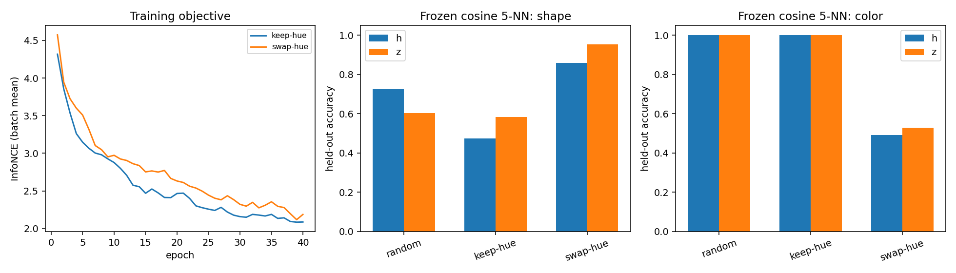
保色条件的 InfoNCE 从 4.317 降至 2.087,但 h 的形状 5-NN 从随机的 72.50% 降到 47.50%。目标可以利用颜色、位置、大小来区分源图;目标下降没有回答形状类别是否更可分。线性形状读出却从 56.25% 增至 69.17%,说明同一表示在不同读出协议下也会得出不同评价。
换色条件的 h 形状 5-NN 为 85.83%,颜色 5-NN 为 49.17%;形状线性读出为 98.75%,颜色线性读出仍有 59.17%,说明不能把“近邻接近50%”升级成数学意义的信息完全消失。z 的形状 5-NN 达到 95.42%,这次反而高于 h;“下游总用 h,因为 h 总更好”不是本实验支持的规则。
两条链的第一层卷积权重变化范数分别为 0.7133 和 0.7588,确认不是只训练了读出头。这里不能证明大规模自然图像上颜色增强总能提高形状识别,也不能从一枚种子宣称显著优越。
云端复核(2026-09-22):同一代码另在 Deepnote 的 Python 3.13 / PyTorch 2.12.0+cu130 环境以 CPU 张量完整执行。保色 h 的形状/颜色5-NN为54.17%/100%,换色为93.33%/50.42%;本地表格来自 Python 3.12 / PyTorch 2.14 CPU,保留原值。固定种子不保证跨软件版本逐位相同;这里两次都显示形状与颜色任务的取舍。云端运行 ID:5c5da87a-d3b9-4a10-b758-269e659f54f1。
只改一个条件,再解释变化
先保持数据、网络、epoch 与读出协议,修改 views 中色相交换概率,从 0.5 改成 0.1。把结果写入新的输出目录,保留原基准;观察颜色线性读出是否恢复、形状读出是否变化。不要同时增加模型和训练时长。若增加一个颜色敏感下游任务,例如“成熟红果与未熟绿果”,请先说明哪些增强可能直接改掉答案。
来源:SimCLR 原论文与作者发布页 支持增强组成、非线性投影头和冻结评价的研究背景。本册图形数据、CPU 小网络、对照结果为本课程独立教学构造,不是论文 ImageNet 指标复现。